Development of a Four-Dimensional Diagnostic Analysis Model for Assessing Ensemble Forecast Uncertainty

1.   Introduction

Due to the chaotic nature of atmospheric motions, initial errors of numerical models, as well as errors in the models themselves, it is inevitable that errors (i.e., uncertainties) also exist in numerical forecasts, which is one of the central problems affecting the accuracy of weather prediction (Lorenz, 1963; Toth et al., 2001; Zhu, 2005; Mu et al., 2011; Bauer et al., 2015; Chen and Li, 2020). How to quantify and understand forecast uncertainty is extremely important for different users and decision-making services, and a complete forecast should include a quantitative estimate of its uncertainty (Toth et al., 2001, 2007; Zhu et al., 2023). As mentioned above, forecast uncertainty primarily stems from initial errors and model errors. In this respect, by reasonably introducing initial and model perturbations into the model integration processes and running the slightly perturbed model multiple times, ensemble forecasts can make use of the generated perturbed forecasts to provide a probability density distribution of the possible future atmospheric states (Buizza et al., 2005; Chen and Li, 2020). Currently, ensemble forecasting is not only one of the major approaches to estimating forecast uncertainty (Molteni et al., 1996; Zhu et al., 2002; Buizza et al., 2005; Du and Chen, 2010), but can also be used to assess the atmospheric predictability (Zhu et al., 2019a; Zhu, 2020), provide users with probabilistic forecast information that is not available in single-deterministic forecasts (Du and Chen, 2010; Duan et al., 2019), improve the forecasting skill for extreme weather events (Guan and Zhu, 2017; Lee et al., 2020; Peng et al., 2024), and generate decision-making services for users that possess greater economic benefits (Zhu et al., 2002; Peng et al., 2024).

Ensemble forecasts have become a key component of the forecasting operations at most of the world’s major numerical prediction centers, such as ECMWF (Lang et al., 2023), NCEP (Zhou et al., 2022), the Meteorological Service of Canada (McTaggart-Cowan et al., 2022), the Met Office (UKMO; Sanchez et al., 2016), and the China Meteorological Administration (CMA; Chen and Li, 2020). Given that an important value of ensemble forecasting is its ability to provide estimates of the flow-dependent forecast uncertainty (Toth et al., 2001; Zhu et al., 2002; Hopson, 2014), it is necessary to perform a diagnostic analysis on the ability to capture forecast uncertainty when evaluating the strengths and weaknesses of an ensemble prediction system (EPS). Herrera et al. (2016) investigated the forecast uncertainty characteristics of operational global EPSs from eight numerical centers, including ECMWF, NCEP, UKMO, and CMA, by using data for January–February 2012 from the THORPEX Interactive Grand Global Ensemble (TIGGE; Swinbank et al., 2016). They found that there was an obvious difference between the abilities of various operational EPSs to quantitatively estimate forecast uncertainty, and the estimated uncertainties were shown to vary greatly in some local regions. In terms of the diagnosed deficiencies of different operational EPSs in representing forecast uncertainty, Herrera et al. (2016) further discussed the corresponding reasons behind them, comprising the deficiencies associated with the adopted models and the shortcomings of the EPSs in dealing with the initial and model uncertainty. As an update to the work of Herrera et al. (2016), Loeser et al. (2017) employed the data for January–February 2015 from TIGGE to assess the abilities of six major global operational ensembles to predict the spatial and temporal evolution of forecast uncertainty. They pointed out that, apart from the UKMO EPS, all of the examined operational EPSs showed little change in the main characteristics of the simulated forecast uncertainty during 2012–2015, and the ECMWF EPS generally provided the best simulation capability.

Objectively quantifying and evaluating whether an EPS can effectively capture forecast uncertainty helps to clarify the deficiencies of the ensemble perturbation methods and/or the model systems, and thus promote the research and development of EPSs and improvements in model performance (Herrera et al., 2016; Loeser et al., 2017; Zhu et al., 2019b, 2023). To date, a range of methods and metrics have been developed to describe the forecast uncertainty, such as statistical evaluations of probability distributions that compare probability distributions of forecast outcomes with those of observations, information entropy (Shannon, 1948), the continuous ranked probability score (Hersbach, 2000), Talagrand histograms (Candille and Talagrand, 2005), relative measure of predictability (Toth et al., 2001), and correlation analysis between forecast members and observations. In particular, the root-mean-square error (RMSE) of the ensemble mean, ensemble spread (i.e., the standard deviation around the ensemble mean), and their relationships, is often used as an essential category of metrics to diagnose and analyze the completeness or systematic inadequacy of an EPS in estimating forecast uncertainty. For a perfectly reliable EPS, the ensemble mean RMSE should be equal to the ensemble spread, and then the spread can be utilized to predict the forecast uncertainty (Du, 2002; Fortin et al., 2014; Duan et al., 2019). Generally speaking, the larger (smaller) the ensemble spread, the higher (lower) the forecast uncertainty and the lower (higher) the model predictability (Toth et al., 2001; Grimit and Mass, 2007; Hopson, 2014; Fernández-González et al., 2017). Zhu et al. (2023) evaluated the performance of the NCEP global ensemble forecast system with three different configurations in quantifying forecast uncertainty by analyzing the spatiotemporal distributions of ensemble spread, ensemble mean RMSE, and the ratios between the two measures. It was found that the ensemble built on the coupling of atmospheric, ocean, sea ice, and wave models and optimized stochastic parameterization schemes could better represent the forecast uncertainty, and lead to higher probabilistic forecast skills. Furthermore, they used a linear variance calibration (LVC; Kolczynski et al., 2011) approach to diagnose the correlations between the ensemble variance and the ensemble mean forecast error variance, and explored the flow-dependent characteristics of the spread–error relationship.

Forecast uncertainty changes with the general circulation, and is characterized by temporal and spatial variations. Therefore, it should be diagnosed and analyzed from a total of four dimensions covering both time (one dimension) and space (three dimensions), instead of just using statistical metrics based on spatiotemporal averages. To diagnose and analyze the strengths and weaknesses of an EPS in simulating forecast uncertainty from a multidimensional perspective, we developed a four-dimensional diagnostic analysis model for ensemble forecast uncertainty based on the ensemble mean error and ensemble spread. The aim of this model is to objectively present the ability of EPSs to describe the forecast uncertainty by analyzing the relationships between the ensemble mean RMSE and ensemble spread in terms of the temporal evolution (one-dimensional) and spatial distribution (three-dimensional), and by applying the LVC method. Accordingly, the deficiencies of EPSs in representing the forecast uncertainty and the possible reasons can be diagnosed and clarified, based upon which the related technical parameters associated with the model systems and EPSs can then be adjusted to further optimize the ensemble performance.

The global EPS independently developed by the CMA (CMA-GEPS) has been in operation since December 2018 (Chen and Li, 2020). The initial perturbation technique employed in CMA-GEPS, which is based on singular vectors (SVs), and the model perturbation methods, which include the stochastically perturbed physical tendencies (SPPT) scheme and the stochastic kinetic energy backscatter (SKEB) scheme, are in line with other EPSs in operation at some of the world’s leading numerical prediction centers (Li et al., 2019; Lock et al., 2019; Huo et al., 2020; Peng et al., 2020; Zhou et al., 2022). However, since being launched operationally in 2018, the forecast uncertainty characteristics of CMA-GEPS have not yet been systematically studied. In addition, the discrepancies between CMA-GEPS and other well-known EPSs in representing forecast uncertainty still remain unclear. Therefore, in this study, the forecast uncertainty of CMA-GEPS was first analyzed from a multidimensional viewpoint by using the proposed four-dimensional ensemble forecast uncertainty diagnostic analysis model. In this way, the usefulness and value of the applied diagnostic analysis model can be demonstrated. Then, the forecast uncertainty of CMA-GEPS was compared with that of the ECMWF’s state-of-the-art global ensemble, to comprehensively diagnose the shortcomings of CMA-GEPS and the associated causes, thus providing an objective reference for future research and development of CMA-GEPS.

2.   Data and methodology

2.1   Data

The operational forecast data of CMA-GEPS from 1 December 2022 to 30 November 2023 initialized daily at 1200 UTC are adopted with an output frequency of 12 h and a forecast length of 15 days. The examined variables comprise 500-hPa geopotential height (H500) and temperature (T500), 850-hPa zonal wind (U850), and 250-hPa zonal wind (U250). During the study period, the operational version of CMA-GEPS was CMA-GEPS V1.3, which has been in operation since 20 September 2022. Its detailed parameter configuration is listed in Table 1. The forecast model is based on the CMA Global Forecast System (CMA-GFS) V3.3 (Shen et al., 2023), with a horizontal resolution of 0.5° × 0.5° and a time step of 600 s. The initial field of the control forecast is created by interpolating the high-resolution (0.25° × 0.25°) analysis field from the CMA operational global four-dimensional variational (4DVar) data assimilation system (CMA-4DVar; Huo et al., 2018; Zhang et al., 2019). The SVs method is applied to represent the effects of initial analysis errors on forecast uncertainty. Specifically, 15 initial perturbations are produced by linearly combining three sets of SVs using a Gaussian sampling technique (Li et al., 2019; Huo et al., 2020), in which the first set comprises 30 leading SVs targeting the extratropical region of the Northern Hemisphere (30°–80°N), the second set also comprises 30 leading SVs but for the extratropical region of the Southern Hemisphere (80°–30°S), and the third set depends on up to 6 tropical cyclones observed in the Northwest Pacific with around 5 leading SVs for each tropical cyclone. Subsequently, 30 perturbed initial fields are formed by taking the initial field of the control forecast minus and plus these 15 initial perturbations. The impacts from model errors on the forecast uncertainty are captured by using the SPPT and SKEB schemes (Li et al., 2019; Peng et al., 2020). Consequently, CMA-GEPS consists of 1 control forecast and 30 perturbed forecasts with an ensemble size of 31.

Table  1.  Configuration of the operational CMA-GEPS in the period from 1 December 2022 to 30 November 2023

Download as CSV

Item	Setting
Forecast model	CMA-GFS V3.3
Horizontal resolution/ 　vertical levels	0.5° × 0.5°/87 levels (with a model top of 　0.1 hPa)
Initial field of the 　control forecast	Interpolating the high-resolution analysis 　field from the operational CMA-4DVar
Model time step	600 s
Initial perturbation	SVs
Model perturbation	SPPT and SKEB
Ensemble size	31
Forecast length	15 days

 | Show Table

DownLoad: CSV

In order to benchmark the performance of CMA-GEPS with other operational EPSs at the world’s most advanced numerical prediction centers, the forecast data of the ECMWF EPS from 1 December 2022 to 30 November 2023 initialized daily at 1200 UTC are also employed. Different from the ensemble perturbation techniques of CMA-GEPS, ECMWF uses a hybrid initial perturbation method based on SVs and ensemble data assimilation (Buizza et al., 2008; Leutbecher and Palmer, 2008; Lang et al., 2019), and a model perturbation approach based on the multiscale SPPT scheme (Shutts et al., 2011). Over the study period, the horizontal resolution of the ECMWF ensemble forecast model (18 km until June 2023 and 9 km thereafter) was much higher than that of CMA-GEPS. However, due to storage space limitations, the ECMWF ensemble forecast data used in this paper have a relatively coarse horizontal resolution (i.e., 2° × 2°), and contain 1 control forecast and 50 perturbed forecasts with an ensemble size of 51. The output frequency and the forecast length are 24 h and 15 days, respectively. Besides, the verified variables for comparison are composed of H500 and U500 over the Northern Hemisphere extratropical region and U500 and T500 over the tropical region.

2.2   Methodology

2.2.1   Diagnostic and evaluation metrics

The metrics used for diagnosis and evaluation in this study include the ensemble spread, the RMSE of the ensemble mean, as well as their ratios, the ensemble variance, and the ensemble mean error. Assuming that the initialization time is t, the ensemble spread (S_t,i,j,d) at any grid point (i, j) for a given forecast lead time of d can be defined by the following Eqs. (1) and (2):

Here, M represents the ensemble size, and m denotes the mth ensemble member; i and j stand for the geographical location of a grid point, indicating longitude and latitude, respectively; F and EM are the forecasts of an ensemble member and the ensemble mean, respectively.

The ensemble variance (V_t,i,j,d) is equivalent to the square of the ensemble spread S_t,i,j,d:

The ensemble mean forecast error (ERR_t,i,j,d) is calculated by using the model’s own analysis field as the “truth”:

where A_t+d,i,j is the analysis field at the validation time of t + d.

For the lead time of d, the spatiotemporally averaged ensemble spread (SPD_d) and RMSE of the ensemble mean (RMSE_d) are computed by using the area-weighted method according to the following Eqs. (5)–(7):

Here, t₁ and t₂ represent the beginning and the end of the study period, respectively, and NT denotes the total number of the forecast initialization times; i₁ (j₁) and i₂ (j₂) are used to highlight the longitudinal (latitudinal) ranges of the study region; NI stands for the total number of grid points along a given latitude; ${\omega _j}$ is the cosine value of the latitude for a certain grid point, and the sum of ${\omega _j}$ (j = j₁,…, j₂) for all grid points along a given longitude is indicated by W.

To explore the spatial structures of the spread–error relationship, the difference between the ratio of the averaged ensemble spread (AVESPD) to the corresponding RMSE of the ensemble mean (AVERMSE) and its ideal value (1.0), abbreviated as “Ratio,” is defined as follows:

When the spread–error relationship is investigated from the perspective of horizontal distribution, Ratio, AVESPD, and AVERMSE are functions of longitude i, latitude j, and lead time d, and the latter two are chosen as the square roots of the ensemble variance and ensemble mean error’s square averaged over all forecast cases, respectively. That is:

Moreover, if the spread–error relationship is examined from the perspective of vertical distribution, zonal averages are further implemented on the basis of Eqs. (9) and (10). In this situation, Ratio, AVESPD, and AVERMSE are functions of latitude j and lead time d, and the latter two are obtained by using Eqs. (11) and (12) as follows:

The diagnostic metric Ratio aims to quantify the difference between the ensemble spread and RMSE of the ensemble mean. The closer to 0 the value of Ratio is, the more reliable the ensemble is. If Ratio is less than 0, it suggests that the ensemble is underdispersive and the forecast uncertainty is underestimated, and vice versa.

2.2.2   LVC approach

The LVC approach, proposed by Kolczynski et al. (2011), aims to examine the flow-dependent ensemble reliability by analyzing the linear relationship between the ensemble variance and ensemble mean error variance. In this approach, the ensemble variances at a given forecast lead time for all grid points in the study region are sorted in ascending order, and the ensemble mean errors are ranked by the ensemble variances. The sorted ensemble variances are then divided into NB equally populated bins (NB = 1000 in this study), and meanwhile the ranked ensemble mean errors are also divided into NB equally populated bins. Within each bin, the average of the ensemble variances and variance of the ensemble mean errors are calculated. Via this procedure, a scatterplot can be obtained by pairing the ensemble variances and the corresponding ensemble mean error variances in all NB bins. With these ensemble variance–ensemble mean error variance pairs, a linear regression of ensemble mean error variance is performed as a function of ensemble variance to obtain the slope ${\beta _1}$ and the y-intercept ${\beta _0}$. According to the regression dilution theory, the adjusted slope ${{\hat \beta _1}}$ and the adjusted y-intercept ${{\hat \beta _0}}$ are computed to remove the impacts from sampling errors due to the limited ensemble size on the reliability assessments.

For a perfectly reliable ensemble, the values of ${{\hat \beta _1}}$ (${\beta _1}$) and ${{\hat \beta _0}}$ (${\beta _0}$) are 1 and 0, respectively. That is to say, the more the relationship between the ensemble variance and the ensemble mean error variance converges to one-to-one, the better the ability to represent the forecast uncertainty. A more detailed description of the LVC method can be found in Kolczynski et al. (2011).

2.2.3   Four-dimensional diagnostic analysis model for ensemble forecast uncertainty

The four-dimensional diagnostic analysis model for ensemble forecast uncertainty was developed to objectively present the strengths, weaknesses, and problems of EPSs in simulating the forecast uncertainty by analyzing the relationships between the ensemble mean RMSE and the ensemble spread in terms of the temporal evolution (one-dimensional) and spatial distribution (three-dimensional), and by applying the LVC method. The following three aspects are primarily involved:

(1) The temporal evolution of the spread–error relationship is analyzed in terms of spatial averages;

(2) The spatial distribution characteristics of the spread–error relationship are examined;

(3) The linear relationship between the ensemble variance and the ensemble mean error variance is objectively evaluated by using the LVC method.

This four-dimensional diagnostic analysis model aims to utilize multiperspective evaluations to quantify and understand the forecast uncertainty more accurately. By using this model, the limitations of EPSs in representing forecast uncertainty can be identified and employed to provide guidelines for improving the forecast models and adjusting the technical parameters of EPSs, ultimately helping to enhance the forecast quality and the reliability of the decision-making they support.

3.   Results and analysis

3.1   Forecast uncertainty of CMA-GEPS

3.1.1   Temporal evolution of the spread–error relationship

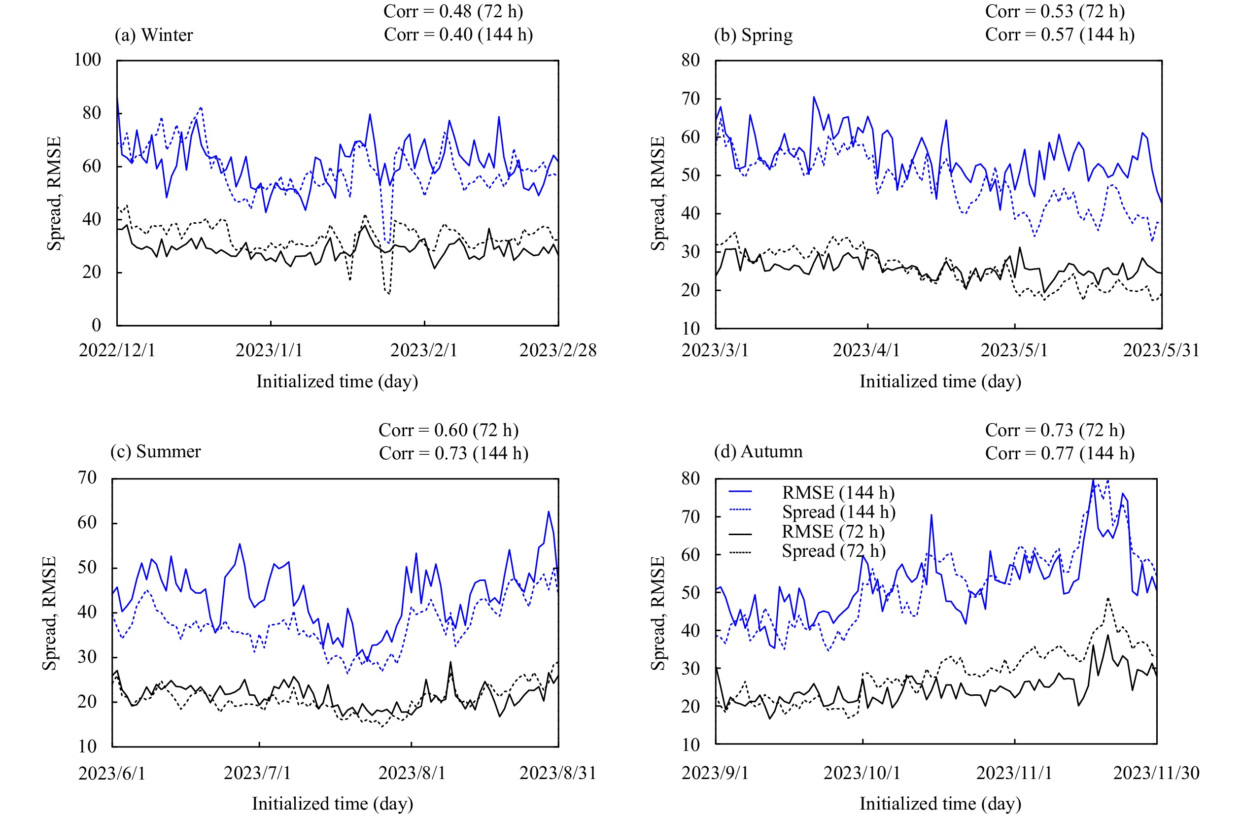
One of the most common methods for evaluating the spread–error relationship of an EPS is to compare the regionally averaged ensemble spread and ensemble mean RMSE, which has an ideal relationship of one-to-one. Figure 1 presents the results for the Northern Hemisphere extratropical region. It can be seen that the spread of H500 is obviously larger than the ensemble mean RMSE at lead times shorter than 108 h, indicating an overdispersion problem with CMA-GEPS; however, the results are reversed for longer forecast lead times beyond 108 h, suggesting an underdispersion deficiency (Fig. 1a). This behavior is consistent with the conclusions of Peng et al. (2023) drawn from the operational forecast data of CMA-GEPS for the period from 1 June 2020 to 31 May 2021. Moreover, as illustrated by Fig. 2, for H500 over the Northern Hemisphere extratropics, the evolution of the ensemble spread with initialization time in different seasons basically tends to be consistent with that of the ensemble mean RMSE. For the short-term (medium-range) forecast lead time of 72 h (144 h), there is a significant positive correlation between the ensemble spread and the ensemble mean RMSE in all of the four seasons comprising winter (Fig. 2a), spring (Fig. 2b), summer (Fig. 2c), and autumn (Fig. 2d), with correlation coefficients of 0.48 (0.40), 0.53 (0.57), 0.60 (0.73), and 0.73 (0.77), respectively. In general, the spread is able to capture the general characteristics of the forecast uncertainty. Despite the above-mentioned problem of overdispersion with respect to annual means at the 72-h lead time, not all of the ensemble forecasts are shown to be overdispersive, depending on the initialization times in different seasons. The larger annual mean spread observed in Fig. 1a is mainly caused by the larger spread in winter, spring, and autumn, while the spread is usually smaller than the ensemble mean RMSE in summer (Fig. 2). Similarly, different from the underdispersive result in terms of the annual means at the 144-h lead time, the ensemble forecasts are found to be overdispersive at some initialization times in winter and autumn (Figs. 1a, 2a, 2d). For other verified variables in the Northern Hemisphere extratropical region, such as U250, U850, and T850, the ensemble is underdispersive over the entire forecast period, and consequently the forecast uncertainty is underestimated by CMA-GEPS (Figs. 1b–d).

Download

Larger image

PowerPoint slide

Fig  1.  The ensemble spread (dashed lines) and RMSE of the ensemble mean (solid lines) averaged over the Northern Hemisphere extratropical region (20°–90°N) as a function of forecast lead time for (a) 500-hPa geopotential height (H500; gpm), (b) 250-hPa zonal wind (U250; m s⁻¹), (c) 850-hPa zonal wind (U850; m s⁻¹), and (d) temperature (T850; K) from the CMA-GEPS operational system initialized daily between 1200 UTC 1 December 2022 and 30 November 2023.

Download

Larger image

PowerPoint slide

Fig  2.  The ensemble spread (dashed lines) and RMSE of the ensemble mean (solid lines) averaged over the Northern Hemisphere extratropical region (20°–90°N) at the forecast lead times of 72 h (black lines) and 144 h (blue lines) for the 500-hPa geopotential height (gpm) from the CMA-GEPS operational system as a function of initialized time in different seasons: (a) winter, (b) spring, (c) summer, and (d) autumn.

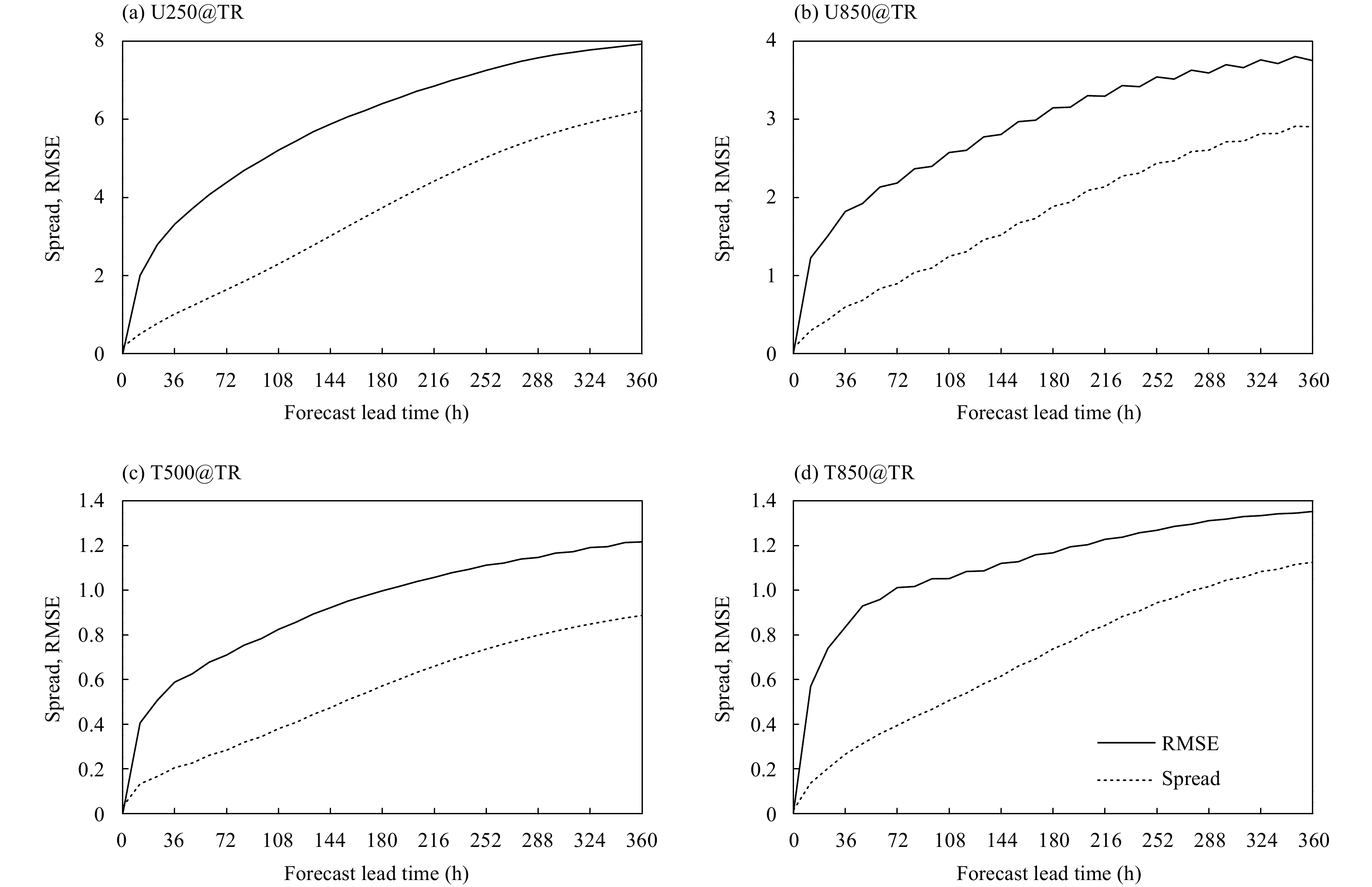
Unlike the Northern Hemisphere extratropical region, the ensemble spread in the tropical region is markedly insufficient compared to the ensemble mean RMSE in the whole forecast range (Fig. 3), which indicates that the forecast uncertainty is underestimated. The reason lies in the limitations of the initial perturbation strategy and insufficient stochastic physical perturbations used by CMA-GEPS. As described in Section 2.1, initial perturbations are generated by linearly combining SVs for the extratropical region of the Southern Hemisphere, the extratropical region of the Northern Hemisphere, and up to six tropical cyclone regions in the Pacific Ocean, using a Gaussian sampling technique. If there are no tropical cyclones in the Pacific Ocean, the initial perturbations in the tropics will be generally absent. This inevitably results in an undersampling problem of the initial uncertainty in the tropical region. Moreover, although the model perturbation schemes (i.e., SPPT and SKEB) can significantly increase the ensemble spread in the tropics (Peng et al., 2020), smaller perturbation amplitudes are always applied to ensure the numerical stability of the operational system, which is also not conducive to the effective representation of forecast uncertainty in the tropics for CMA-GEPS.

Download

Larger image

PowerPoint slide

Fig  3.  The ensemble spread (dashed lines) and RMSE of the ensemble mean (solid lines) averaged over the tropical region (20°S–20°N) as a function of forecast lead time for (a) 250-hPa zonal wind (U250; m s⁻¹), (b) 850-hPa zonal wind (U850; m s⁻¹), (c) 500-hPa temperature (T500; K), and (d) 850-hPa temperature (T850; K) from the CMA-GEPS operational system initialized daily between 1200 UTC 1 December 2022 and 30 November 2023.

3.1.2   Spatial distribution of the spread–error relationship

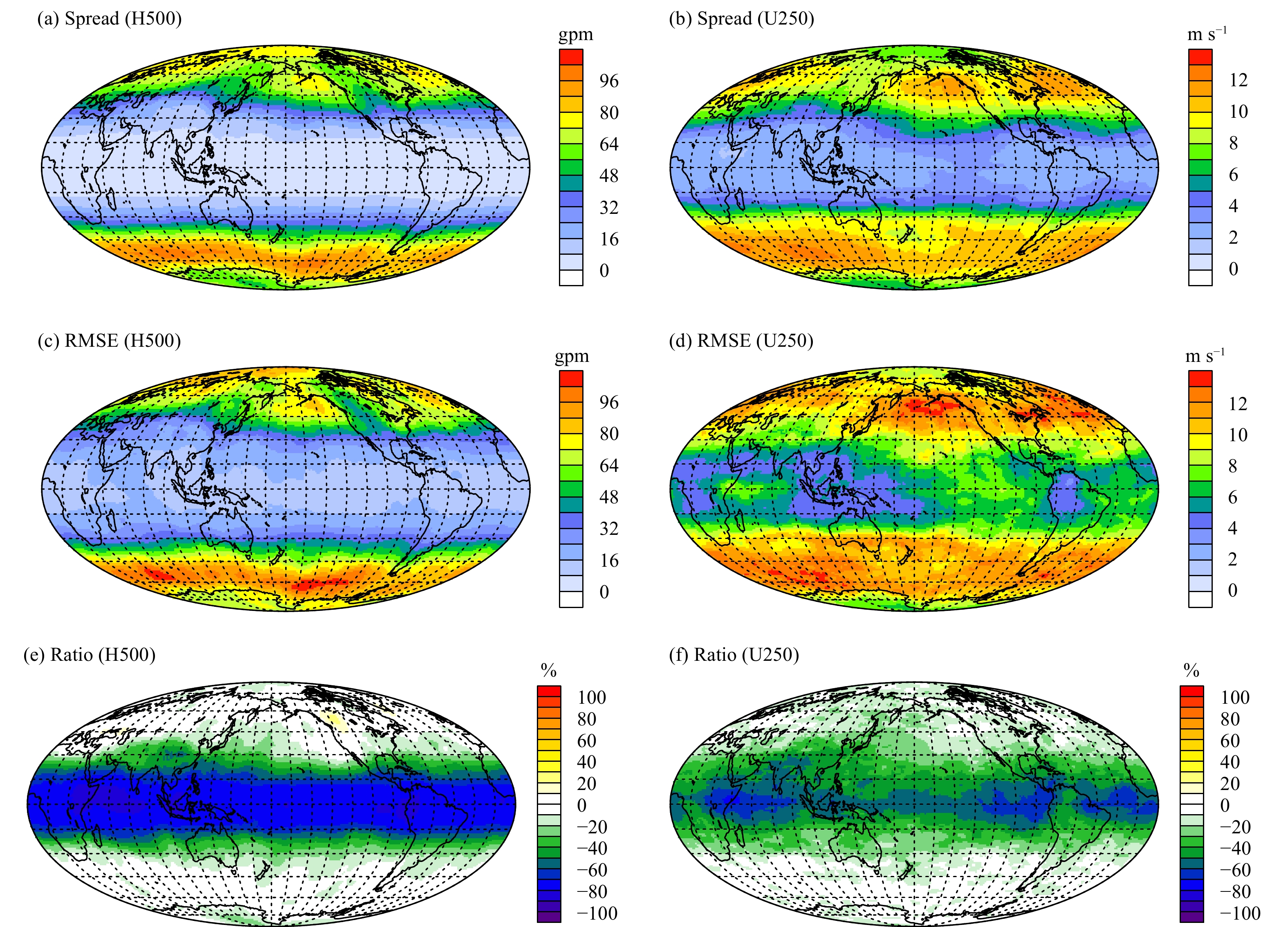
In addition to regional averages, a more detailed diagnostic analysis of the point-to-point spread–error relationship is included from the perspective of three-dimensional spatial distributions. For statistically consistent ensembles, the ensemble spread and the ensemble mean RMSE should be the same in both spatial structure and magnitude. Figure 4 displays the horizontal distributions of the ensemble spread, the ensemble mean RMSE, and the diagnostic metric Ratio for H500 and U250 at the 144-h forecast lead time. By definition, the closer to 0 the value of Ratio is, the higher the ensemble reliability and the better the ability of an EPS to simulate the forecast uncertainty. Also, a positive (negative) value of Ratio means that the spread is larger (smaller) than the RMSE and the forecast uncertainty is overestimated (underestimated). Overall, the horizontal structures of the spread and the RMSE are in good agreement for the different examined variables, with smaller absolute values in the tropics and larger absolute values in the extratropics (Figs. 4a–d). The diagnostic metric Ratio, designed to quantify the difference between the spread and the RMSE, typically varies between −20% and 20% in the extratropics, while it is generally less than −50% in the tropics (Figs. 4e, f). These results suggest that CMA-GEPS is obviously better at representing the forecast uncertainty in the extratropics than in the tropics. Moreover, in the tropics, the values of Ratio for U250 are closer to 0 than they are for H500, and thus the forecast uncertainty in U250 can be represented more accurately. The previous section showed that the regionally averaged spread of H500 is smaller than the RMSE at the 144-h forecast lead time (Fig. 1a), but there are still some local regions, such as the west of North America, where the spread is larger than the RMSE (Fig. 4e). Therefore, more information on the spread–error relationship could be detected via a diagnostic analysis of the spatial distributions.

Download

Larger image

PowerPoint slide

Fig  4.  Horizontal distributions of (a, b) the ensemble spread (gpm and m s⁻¹, respectively), (c, d) the RMSE of the ensemble mean (gpm and m s⁻¹, respectively), and (e, f) the diagnostic metric Ratio (%), which represents the difference between the ratio of the ensemble spread to the RMSE of the ensemble mean and the ideal value of 1.0, at the 144-h forecast lead time for 500-hPa geopotential height (H500; left column) and 250-hPa zonal wind (U250; right column) from the CMA-GEPS operational system initialized daily between 1200 UTC 1 December 2022 and 30 November 2023.

Figure 5 depicts the vertical distributions of the diagnostic metric Ratio at the lead time of 144 h. It can be seen that the values of Ratio in the extratropics are close to the ideal value of 0 for the mass field (geopotential height), the dynamical field (zonal wind), and the thermal field (temperature) at different isobaric pressure levels; however, in the tropics, the Ratio values are far from the ideal value 0 and thus the forecast uncertainty is seriously underestimated. Moreover, as the vertical height increases, the latitudinal range with the spread apparently smaller than the RMSE is extended poleward. As a result, CMA-GEPS is able to capture the forecast uncertainty of the lower-level variables better than the higher-level variables. In contrast to the mass and thermal fields, the values of Ratio for the dynamical field are generally closer to 0, and the forecast uncertainty can be better represented.

Download

Larger image

PowerPoint slide

Fig  5.  Latitude–height cross-sections of the diagnostic metric Ratio (%), which represents the difference between the ratio of the ensemble spread to the RMSE of the ensemble mean and the ideal value of 1.0, at the 144-h forecast lead time for (a) geopotential height (H), (b) zonal wind (U), and (c) temperature (T) from the CMA-GEPS operational system initialized daily between 1200 UTC 1 December 2022 and 30 November 2023.

3.1.3   Linear relationship between ensemble variance and error variance

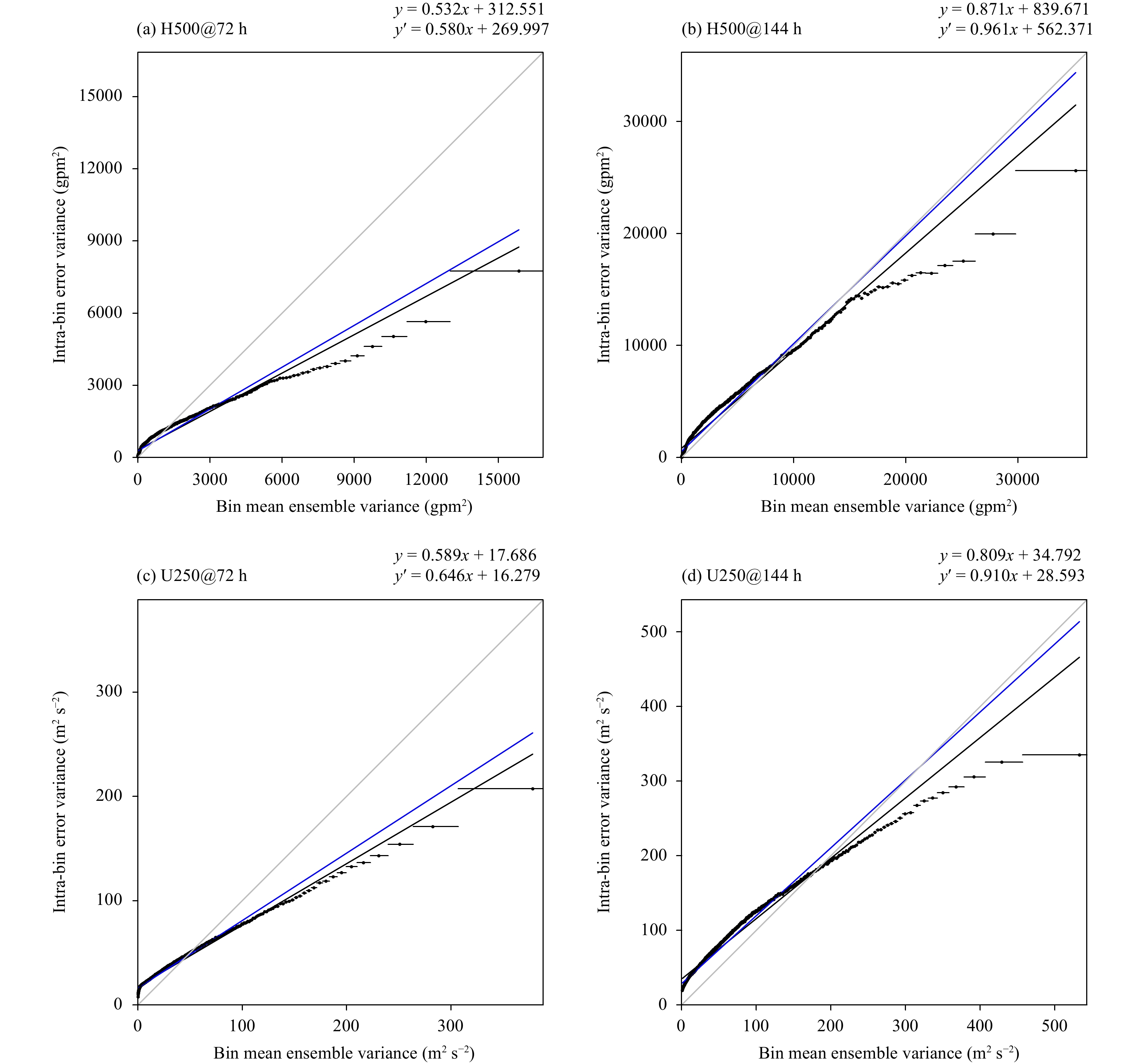
The ensemble variance can be seen as a measure of the forecast error variance, also providing a representation of forecast uncertainty (Wang and Bishop, 2003; Wang et al., 2004; Satterfield and Bishop, 2014). The linear relationship between the CMA-GEPS ensemble variance and the ensemble mean error variance is evaluated by using the LVC method in this part. In terms of H500 and U250 at the representative lead times of 72 and 144 h, the ensemble mean error variance in each bin as a function of the mean ensemble variance is displayed as black points in Fig. 6. It can be observed that, with respect to the different variables, for small (large)-ensemble variance bins, the small (large) ensemble variance generally maps to relatively larger (smaller) ensemble mean error variance, and in this case the forecast uncertainty is underestimated (overestimated). For example, when the ensemble variance of U250 at the 72-h lead time is smaller (larger) than about 49.0 m² s⁻², the ensemble mean error variance is larger (smaller) compared to the corresponding ensemble variance (Fig. 6c), indicating underestimation (overestimation) of the forecast uncertainty. This phenomenon may be related to the limited ensemble size and the incompleteness of the forecast model itself.

Download

Larger image

PowerPoint slide

Fig  6.  Scatterplots of the ensemble mean error variance as a function of the ensemble variance for each of the 1000 bins in terms of the (a, b) global geopotential height at 500 hPa, and (c, d) zonal wind at 250 hPa, at the lead times of (a, c) 72 h and (b, d) 144 h, from the CMA-GEPS operational system, as well as the linearly fitted lines from the LVC method before (black lines) and after (blue lines) impacts from the limited ensemble size were removed. Horizontal lines indicate the ranges of ensemble variance contained in each bin. For the equations presented in the upper-right corner of each subplot, x represents the independent variable (specifically, the bin mean ensemble variance), while y and y' denote the black and blue fitted lines, respectively.

In addition, prior to calibrations for eliminating the impacts of the limited ensemble size on reliability, the ensemble variance–error variance pairs (black points in Fig. 6) can be linearly fitted by the black lines in Fig. 6, of which the slopes ${\beta _1}$ are less than 1 at different lead times and the y-intercepts ${{\beta _0}}$ are greater than 0. Moreover, the slope ${\beta _1}$ increases with the forecast lead time. For H500 (U250), it increases from 0.532 (0.589) at 72 h to 0.871 (0.809) at 144 h. This suggests that, with the increase in forecast lead time, the linear relationship between the ensemble variance and the ensemble mean error variance becomes closer to one-to-one, and the reliability of CMA-GEPS is improved, thus alleviating the problem of the inaccurate representation of forecast uncertainty. After adjustments for the limited ensemble size according to the theory of regression dilution [see appendix from Kolczynski et al. (2011)], the fitted lines are changed to the blue lines of Fig. 6. Apparently, the adjusted slopes ${{\hat \beta _1}}$ are increased compared with the previous ones. At 72 h, the adjusted slope ${{\hat \beta _1}}$ is 0.580 for H500 and 0.646 for U250; and at 144 h, the values even exceed 0.9 (0.961 for H500 and 0.910 for U250), closer to the ideal value of 1. Hence, under the current technical parameters of CMA-GEPS, an increase in the ensemble size can improve its reliability, and contribute to a better representation of forecast uncertainty. However, such an increase in the ensemble size will mean greater computational and storage resource costs, which will need to be considered carefully if implemented operationally.

3.2   Comparison between CMA-GEPS and ECMWF EPS

3.2.1   Spread–error relationship as a function of forecast lead time

To compare CMA-GEPS with a state-of-the-art EPS regarding the ability to represent forecast uncertainty, a diagnostic analysis with the ECMWF EPS was further performed. As the horizontal resolution of the ECMWF EPS data we were able to access (i.e., 2° × 2°) was lower than that of the CMA-GEPS data (i.e., 0.5° × 0.5°), the original CMA-GEPS data were bilinearly interpolated to the same resolution as the ECMWF EPS data for a fair comparison. Based on the interpolated data, the spread and the ensemble mean RMSE were recalculated for CMA-GEPS. Note that the lower-resolution data were only used for comparisons between the CMA and EC-MWF EPSs.

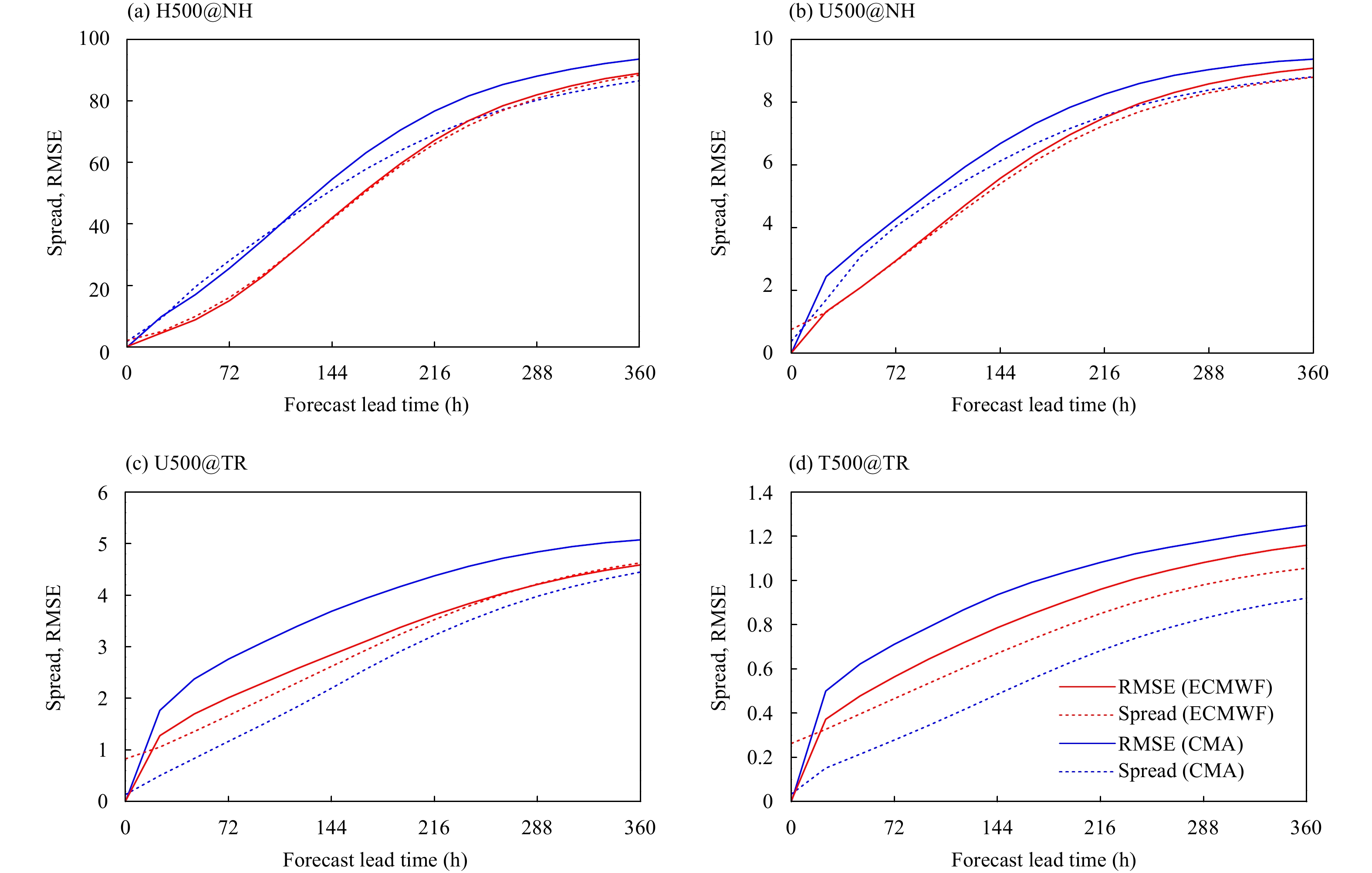
Figure 7 shows the domain-averaged ensemble spread and ensemble mean RMSE for both EPSs. In the Northern Hemisphere extratropical region, the spread and RMSE of H500 from the ECMWF EPS are nearly the same at all lead times (Fig. 7a), while the spread of U500 is slightly smaller than the RMSE only for lead times beyond 96 h (Fig. 7b). On the whole, the ECMWF EPS is able to reliably simulate the forecast uncertainty. Compared with the ECMWF EPS, the RMSE and spread of CMA-GEPS are larger, and the difference between the two is more obvious, particularly in the latter part of the forecast range. In the tropics, although both EPSs share the problem of underdispersion with the spread smaller than the RMSE, the spread–error relationship in the ECMWF EPS is more reasonable (Figs. 7c, d). Additionally, the RMSE of CMA-GEPS is still larger than that of the ECMWF EPS, but the spread is smaller. The former is mainly related to the larger errors of the CMA model itself, while the latter can be explained by the fact that the ECMWF EPS uses an initial perturbation technique based on SVs and ensemble data assimilation, which can reasonably sample the initial uncertainty in the tropics and make the initial ensemble spread of the ECMWF EPS significantly larger than that of CMA-GEPS (see the red and blue dashed lines in Figs. 7c, d). Due to the better match between the spread and RMSE, the ECMWF EPS can represent the forecast uncertainty more accurately than CMA-GEPS.

Download

Larger image

PowerPoint slide

Fig  7.  The ensemble spread (dashed lines) and RMSE of the ensemble mean (solid lines) averaged in the Northern Hemisphere extratropical region (20°–90°N) for (a) 500-hPa geopotential height (H500; gpm) and (b) zonal wind (U500; m s⁻¹), and in the tropical region (20°S–20°N) for (c) 500-hPa zonal wind (U500; m s⁻¹) and (d) temperature (T500; K), as a function of forecast lead time, from the CMA (blue lines) and ECMWF (red lines) operational global EPSs initialized daily between 1200 UTC 1 December 2022 and 30 November 2023.

3.2.2   Spread–error growth as a function of forecast lead time

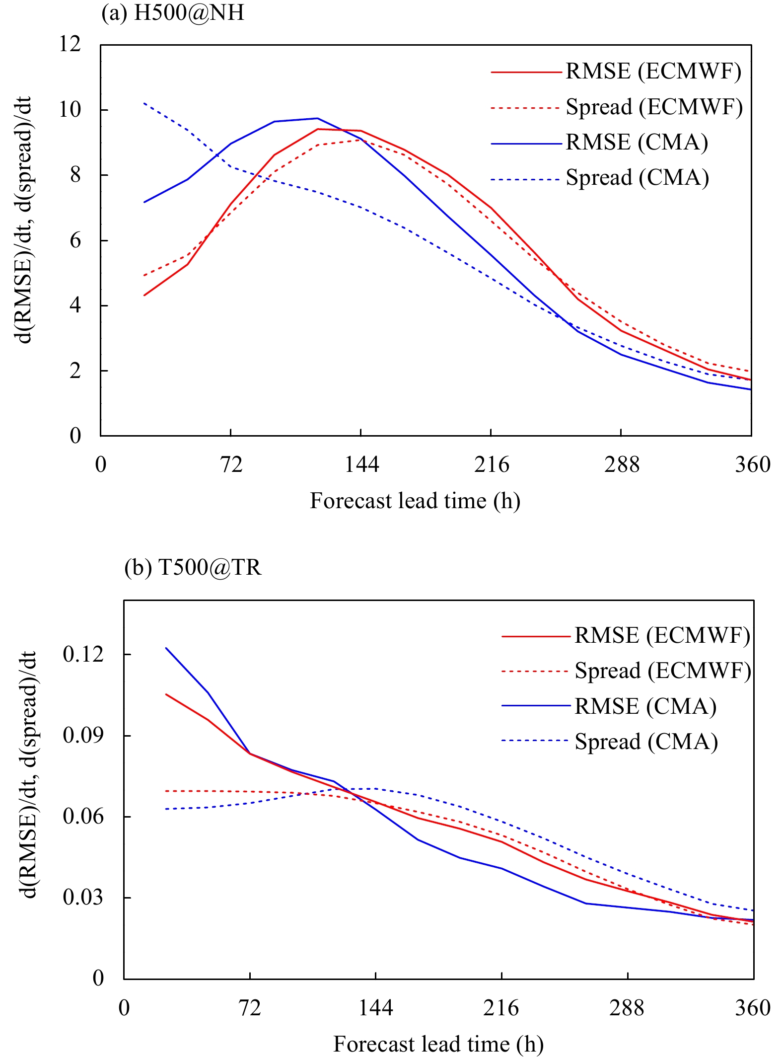
For a perfect EPS, since the ensemble spread is equal to the ensemble mean RMSE at all forecast lead times, the spread and RMSE should grow at the same rate (Berner et al., 2009). In the Northern Hemisphere extratropical region, the consistency between the growth rates of the spread and RMSE from CMA-GEPS is inferior to that from the ECMWF EPS (Fig. 8a). Taking H500 as an example, the growth rate of the RMSE from CMA-GEPS, and that of the spread and RMSE from the ECMWF EPS, show similar characteristics, which increase for short lead times until the maximum values are reached, and gradually decrease thereafter. This growth process is reasonable, and has been reported in many studies (e.g., Dalcher and Kalnay, 1987; Herrera et al., 2016). However, the growth of the spread for H500 from CMA-GEPS presents different characteristics: it decreases all the time during the whole forecast range. The main reason is that the magnitudes of the initial perturbations of CMA-GEPS in the extratropics are too large, leading to the fastest spread growth initially, and this is also supported by the overdispersion of H500 for lead times shorter than 108 h (Fig. 1a). Furthermore, the RMSE (spread) of CMA-GEPS grows faster than that of the ECMWF EPS at lead times shorter than 144 h (96 h), but grows slower for the longer lead times. In the tropics, the evolution of the growth rate for the spread and RMSE of T500 from CMA-GEPS is consistent with that of the spread and RMSE from the ECMWF EPS, respectively (Fig. 8b). Besides, the RMSE of CMA-GEPS grows faster than that of the ECMWF EPS up to 144 h, but grows slower thereafter. Different from the RMSE, the spread of CMA-GEPS grows slower at the beginning, and faster than that of the ECMWF EPS for lead times beyond 96 h. Nevertheless, because the initial spread is smaller, the spread of CMA-GEPS is smaller than that of the ECMWF ensemble (Fig. 7d).

Download

Larger image

PowerPoint slide

Fig  8.  Growth rates of the ensemble spread (dashed lines) and RMSE of the ensemble mean (solid lines) averaged (a) in the Northern Hemisphere extratropical region (20°–90°N) for 500-hPa geopotential height [H500; gpm (24 h)⁻¹], and (b) in the tropical region (20°S–20°N) for 500-hPa temperature [T500; K (24 h)⁻¹], as a function of forecast lead time from the CMA (blue lines) and ECMWF (red lines) operational global EPSs initialized daily between 1200 UTC 1 December 2022 and 30 November 2023.

In summary, the differences in the RMSE and spread between CMA-GEPS and ECMWF EPS are not only closely related to the ensemble perturbation technique, but also to the performance of the forecast model itself. It should be noted that, in different regions, the more rapid growth of the CMA-GEPS RMSE relative to that of ECMWF EPS for the initial 24-h forecast period, may be caused by the inconsistency between the model and the initial fields (Figs. 7, 8). Buizza et al. (2005) and Palmer (2019) pointed out that the performance of EPSs strongly depends on the quality of the data assimilation system that forms the initial fields of the control forecasts, as well as the performance of the numerical model itself that produces the forecasts. Therefore, the coordination between the forecast model and the assimilation system of CMA needs to be urgently optimized in order to narrow the gap between the CMA and ECMWF EPSs.

4.   Summary and discussion

For objectively evaluating the ability of EPSs in representing forecast uncertainty, a four-dimensional diagnostic analysis model for ensemble forecast uncertainty was developed. The model works by analyzing the relationships between the ensemble spread and the ensemble mean RMSE from the perspective of the temporal evolution (one-dimensional) and spatial distribution (three-dimensional), and by applying the LVC method. Then, with the help of the EPSs’ diagnosed deficiencies in representing the forecast uncertainty and the possible reasons behind, adjustments to the relevant technical parameters of EPSs and their forecast models could be determined and implemented, thus contributing to the continuous improvement and development of EPSs. In the present study, this four-dimensional diagnostic analysis model was applied to CMA-GEPS by using the daily operational forecast data in a 1-yr period from 1 December 2022 to 1 November 2023. Also, comparisons were made between CMA-GEPS and the ECMWF EPS to clarify the deficiencies of CMA-GEPS in estimating the forecast uncertainty and the related reasons. The main conclusions are summarized as follows.

(1) From the evolution of the spatiotemporally averaged spread–error relationship with forecast lead time, the ensemble spread of CMA-GEPS in both the extratropical and tropical regions is generally smaller than the ensemble mean RMSE, indicating an underestimation of forecast uncertainty. Relative to the extratropical region, the underestimation of forecast uncertainty in the tropical region is more serious, which is closely related to deficiencies in the initial and model perturbation methods utilized by CMA-GEPS. In terms of the regionally averaged spread–error relationship as a function of the initialized time in different seasons and its spatial distribution, the deficiency of underestimating the forecast uncertainty does not exist everywhere. For example, in some seasons and local regions, the ensemble spread is greater than the ensemble mean RMSE, suggesting that the phenomenon of overestimated forecast uncertainty also exists. Moreover, CMA-GEPS performs better in describing the uncertainty in lower-level variables than upper-level variables; and compared with the mass field and thermal field, the forecast uncertainty of the dynamic field is better captured.

(2) The results from the LVC method reveal that the linear relationship between the ensemble variance and ensemble mean error variance of CMA-GEPS is improved as the forecast lead time increases, and the deficiency in terms of the underestimation of forecast uncertainty is continuously alleviated. With the current technical parameters of CMA-GEPS, more ensemble members can lead to a better representation of forecast uncertainty to some degree.

(3) The spread–error relationship of CMA-GEPS is not as good as that of the ECMWF EPS; and in the ECMWF EPS, the representation of forecast uncertainty is more reasonable and accurate. The ensemble mean RMSE of CMA-GEPS is usually larger than that of the ECMWF EPS in different regions. Also, the ensemble spread of CMA-GEPS is larger than that of the ECMWF EPS in the extratropical region, while it is smaller in the tropical region. Overall, CMA-GEPS suffers from lower consistency and reliability. Diagnostic analysis of growth rates revealed that the growth processes of the spread and RMSE in the extratropical region are not well matched for CMA-GEPS, while the opposite is true for the ECMWF EPS. Regarding CMA-GEPS, the reason for the mismatch between the spread and error growth processes lies in that the adopted initial perturbation magnitudes are too large in the extratropical region, making the spread grow too fast at the first few lead times. In the tropical region, the spread and error growth processes in CMA-GEPS are consistent with those in the ECMWF EPS, and the slower spread growth of CMA-GEPS in the short forecast range is primarily due to the undersampled initial errors in this region.

To sum up, CMA-GEPS generally underestimates the forecast uncertainty. Compared with the ability of the ECMWF EPS in capturing the forecast uncertainty, a considerable gap exists for CMA-GEPS. On the one hand, the reason for this gap is related to the relatively large error of the CMA-GEPS forecast model itself; on the other hand, it is related to the deficiencies in the methods employed to generate the initial and model perturbations, as well as the smaller ensemble size. In future work, if the ensemble perturbation generation technique can be further optimized on the basis of reducing the model error itself, CMA-GEPS will be able to better quantify the forecast uncertainty information.

Finally, it should be noted that the four-dimensional diagnostic analysis model constructed in this study is not limited to just evaluating global EPSs. It can be adapted to diagnose any ensemble system, including convective-allowing ensembles, seasonal EPSs, and even multimodel ensembles. In the future, more metrics and methods will be incorporated into the four-dimensional diagnostic analysis model to extract more useful information about forecast uncertainty.